Water withdrawals and allocation

The native daily managed-water layer represents surface-water diversions, groundwater pumping, sector demands, consumption, delayed returns, a conceptual aquifer and an optional reservoir. It works with daily hydrological models, single-basin and multi-basin calibration, Morris/Sobol sensitivity and reports. No CWatM, Pywr, PCRaster or MODFLOW installation is required.

Available since version 0.2.0. Install with python -m pip install basinforge-hydro==0.2.0.

Units and inputs

All managed-water flows are m³ per daily step, not m³/s. Storage and capacities are m³. Multiply discharge in m³/s by 86,400. Convert model runoff in mm/day to volume using q_mm * basin.area_km2 * 1000. Dates must be contiguous, timezone-naive daily dates. Inputs are nonnegative scalars or arrays with one value per day. Invalid/missing forcings are refused.

Measured withdrawals are preferable. Where they are unavailable, supply explicitly labelled demand scenarios. Rainfall and outlet discharge do not uniquely identify pumping, irrigation, consumption and return-flow parameters.

Run accounting directly

import pandas as pd
from basinforge import WaterDemand, WaterUseConfig, simulate_water_use

dates = pd.date_range("2020-01-01", periods=365)
demands = [
    WaterDemand("domestic", 3000, priority=0, consumption_fraction=0.2),
    WaterDemand("irrigation", 10000, priority=1, consumption_fraction=0.7,
                groundwater_return_fraction=0.5, return_delay_days=7),
    WaterDemand("industry", 2000, source="surface", priority=2,
                consumption_fraction=0.25, return_delay_days=2),
]
config = WaterUseConfig(
    environmental_flow=1000, pumping_capacity=5000,
    baseflow_fraction=0.2, groundwater_recession=0.03,
    groundwater_initial=100000,
)
# Constant natural inflow below is an illustrative scenario, not observations.
result = simulate_water_use(dates, 20000, demands, config)
print(result.summary())
result.daily.to_csv("water-balance.csv")
print(result.sectors["irrigation"])

source can be surface, groundwater or mixed. Mixed users can draw from both sources. max_withdrawal limits each user’s gross daily supply regardless of requested demand. pumping_capacity limits total pumping. Unmet demand is reported, not supplied from an unlimited fictitious groundwater source. Livestock, power generation and other users can be represented with additional WaterDemand records and their own observed/estimated demand series.

Allocation methods

Method	Rule	Suitable use
`priority`	Compiled loop; lower priority number first; surface preferred, groundwater fallback for mixed users	Repeated calibration and scenario runs
`lp`	SciPy/HiGHS linear programming; maximise total supply within each priority group, then minimise pumping while preserving that supply	Competing source restrictions

Priority-mode ties follow input order. LP ties do not guarantee equal percentage satisfaction. Neither method optimises future reservoir operations or represents water rights automatically. Both allocate one day at a time.

LP can improve source allocation: when a mixed user and a surface-only user both request 10 m³ and each source has 10 m³ available, LP can serve both by using groundwater for the mixed user. Greedy surface-first allocation may leave the surface-only user short.

Environmental flow is reserved before surface diversion. When recession is positive, pumping also retains enough aquifer water to meet today’s remaining environmental minimum through baseflow, if physically possible. Deficits are reported if supply is insufficient; future ecological flows are not guaranteed.

Equations and order of operations

Let \(N_t\) be natural-model runoff volume, \(U_t\) upstream inflow, \(f\) the partition fraction, \(J_t\) separately supplied external recharge, \(G_t\) aquifer storage and \(R^g_t,R^s_t\) returns due today. Natural runoff is partitioned:

\[G_t^* = G_{t-1} + fN_t + J_t + R^g_t, \qquad I_t^s=(1-f)N_t+U_t+R^s_t.\]

Aquifer storage exceeding groundwater_capacity spills to surface water. Partitioning avoids counting \(fN_t\) both as river inflow and new groundwater. Do not supply recharge that duplicates the same water already in \(N_t\).

The optional reservoir regulates this surface branch, before aquifer baseflow joins downstream. With reservoir capacity \(C_H\), starting storage \(H\), requested evaporation \(E_t\) and maximum scheduled release \(L_t\):

\[\widetilde H_t=H_{t-1}+I_t^s,\qquad E_t^a=\min(E_t,\widetilde H_t),\]

\[Z_t=\max(0,\widetilde H_t-E_t^a-C_H),\qquad H_t^*=\widetilde H_t-E_t^a-Z_t,\]

\[L_t^a=\min(L_t,H_t^*),\qquad H_t=H_t^*-L_t^a,\qquad S_t=Z_t+L_t^a.\]

Without a reservoir \(S_t=I_t^s\). reservoir_release is an externally specified maximum daily release, not a forecast-based operating policy. Its default is unlimited, giving pass-through behaviour; specify a finite release schedule to retain water. Evaporation is a requested volume capped by available storage.

For environmental minimum \(F_t\) and recession fraction \(k\), available sources for abstraction are:

\[\begin{split}A_t^s=\max(0,S_t-F_t),\qquad G_t^{reserve}=\begin{cases}\max(0,F_t-S_t)/k,&k>0\\0,&k=0,\end{cases}\end{split}\]

\[A_t^g=\min\left(P_t^{max},\max(0,G_t^*-G_t^{reserve})\right).\]

For sector \(i\), demand \(D_{i,t}\), intake capacity \(M_{i,t}\), supplied surface volume \(W^s_{i,t}\) and pumped volume \(W^g_{i,t}\), allocation obeys:

\[0\le W^s_{i,t}+W^g_{i,t}\le\min(D_{i,t},M_{i,t}),\quad \sum_i W^s_{i,t}\le A_t^s,\quad \sum_i W^g_{i,t}\le A_t^g.\]

Forbidden sources have zero withdrawal. LP solves these constraints separately for each priority group using residual resources. For each group it first maximises \(\sum_i(W^s_{i,t}+W^g_{i,t})\), then minimises \(\sum_i W^g_{i,t}\) while fixing that maximum total supply.

Pumping occurs before aquifer recession:

\[B_t=k\left(G_t^*-\sum_iW^g_{i,t}\right),\qquad G_t^{after}=G_t^*-\sum_iW^g_{i,t}-B_t.\]

For consumption fraction \(c_i\), groundwater share of returns \(r_i\) and integer delay \(\ell_i\):

\[W_{i,t}=W^s_{i,t}+W^g_{i,t},\quad C_{i,t}=c_iW_{i,t},\quad R_{i,t}^{generated}=(1-c_i)W_{i,t},\quad D_{i,t}^{unmet}=D_{i,t}-W_{i,t}.\]

\[R^g_{i,t+\ell_i}\mathrel{+}=r_iR_{i,t}^{generated},\qquad R^s_{i,t+\ell_i}\mathrel{+}=(1-r_i)R_{i,t}^{generated}.\]

Delayed returns use explicit queues. Zero-delay returns are delivered after allocation and cannot be withdrawn again within the same day. Surface returns join the downstream outflow; groundwater returns enter aquifer storage, with any capacity overflow spilling to the river. Delays above 36,500 days are refused to bound queue memory.

Pending returns \(T_t\) remain part of system storage even beyond the final day. The checked daily managed-system balance is:

\[\epsilon_t=(G+H+T)_{t-1}+N_t+U_t+J_t-Q_t-\sum_iC_{i,t}-E_t^a-(G+H+T)_t.\]

This checks the managed-water subsystem, not the complete rainfall/PET balance inside every underlying hydrological kernel.

Demand estimation

domestic_demand(population, litres_per_person_day=100) returns \(population\times rate/1000\) m³/day. Rates are user assumptions or supplied measurements; the default is not universally applicable.

irrigation_demand provides a simple climatic estimate:

\[D_t^{irr}=\frac{\max(0,K_{c,t}PET_t-aP_t)\,A_{irr}\,1000}{\eta}.\]

\(A_{irr}\) is km², PET and precipitation are mm/day, \(a\) is effective rainfall fraction and \(\eta\) application efficiency. Crop coefficients may vary daily, including zero outside the growing season. This is not a soil-moisture, paddy-water or crop-yield model. Irrigation water does not feed back into the native model’s soil store. Treat efficiency and consumption/return fractions consistently; do not automatically classify all irrigation losses as consumed.

One-call calibration, sensitivity and reporting

from basinforge import (Basin, CalibrationConfig, WaterDemand, WaterUseConfig,
                        WaterUseScenario, managed_model, run_experiment,
                        managed_accounting)

basin = Basin.from_csv("basin.csv", basin_id="A", area_km2=1200,
                       q_unit="m3/s", timestep="daily")
scenario = WaterUseScenario(
    basin.dates,
    (WaterDemand("domestic", 3000, consumption_fraction=0.2),),
    WaterUseConfig(baseflow_fraction=0.2, groundwater_recession=0.03,
                   groundwater_initial=100000, pumping_capacity=5000),
)
model = managed_model("GR4J", scenarios={"A": scenario})
study = run_experiment(
    basin, model,
    CalibrationConfig(warmup=365, calibration_fraction=0.7,
                      bounds={"x1": (100, 1500), "wu_demand_scale": (0.5, 2)}),
    sensitivity="morris", output="managed-study",
)
accounting = managed_accounting(basin, model, study["fit"].parameters)

The existing DE, LHS and multi-start searches work unchanged. Use sensitivity="sobol" for Sobol indices. Water parameters are:

Parameter	Meaning	Supported range
`wu_demand_scale`	Multiplier on all requested sector demands	0–3
`wu_consumption_scale`	Multiplier on specified consumption fractions	0–1
`wu_baseflow_fraction`	Natural runoff diverted into the conceptual aquifer	0–1
`wu_groundwater_recession`	Fraction of post-pumping aquifer water released daily	0–1

Select explicit bounds/fixed parameters; the full default joint fit is often unidentifiable. Consumption scaling only reduces the specified fractions; change the scenario itself to explore higher fractions. Return delays and sector-specific fractions are scenario settings, not continuous fit parameters. Sensitivity scores use training discharge only, not a water-use observation objective. The numerical water accounting does not validate assumed demands.

Managed one-call outputs additionally include water-balance.csv, water-sectors.csv and water-summary.json. Preserve the scenario inputs with your study: the fit contains their fingerprint but not all original series. For manual report export pass export_report(basin, fit, folder, model=model); the wrapped model cannot be reconstructed from its name alone.

For independent/shared multi-basin fits, supply a mapping containing a scenario for each basin ID and pass the wrapped model to calibrate_many or calibrate_shared. Process workers are supported. Shared-model defaults for partition/recession must agree; demand and other settings may differ by basin. Training records must be scenario-aligned prefixes so stores/returns start from the same initial state. Full validation simulations run continuously.

Connected basins

run_water_network(dates, natural_runoff, scenarios, downstream, travel_days=...) processes basins upstream to downstream. Each basin has one downstream destination or None. Cycles and unknown IDs are refused. Provide local/incremental runoff volumes: full-catchment upstream runoff would double-count water. Integer travel delays retain unarrived outflows as final_transit; a network-wide balance includes that storage. Bifurcations, canal transfers and a network-wide optimisation are not represented.

LuMod forcing case study

From a checkout with the optional example-data dependency:

python -m pip install -e '.[reference]'
python examples/water_withdrawals.py --output water-use-study

This uses LuMod example 2 forcings and discharge with assumed, clearly labelled domestic/industrial/irrigation scenarios. It runs DE, LHS and multi-start calibration; generates Morris sensitivity, hydrographs and accounting exports; runs Morris/Sobol sensitivity for the water parameters; compares priority and LP; and checks a two-basin network. It is not a reconstruction of measured withdrawals at the LuMod catchment.

Executed example

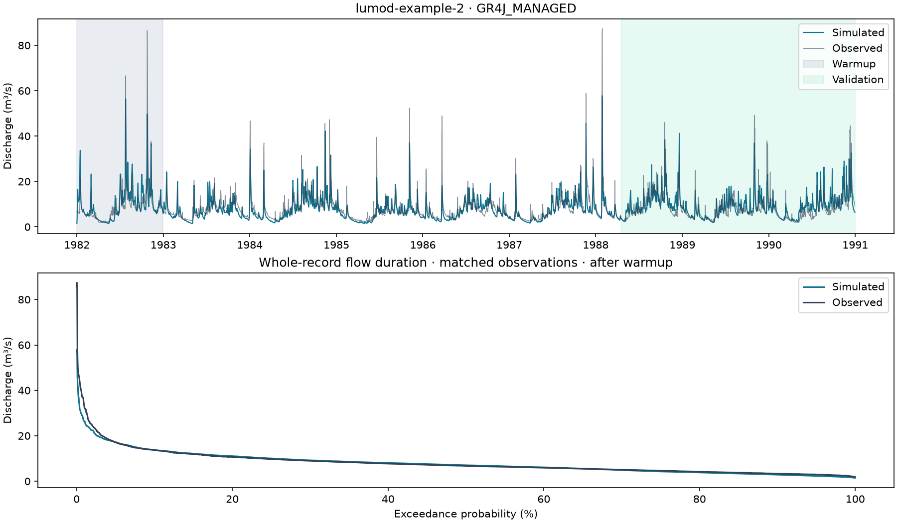
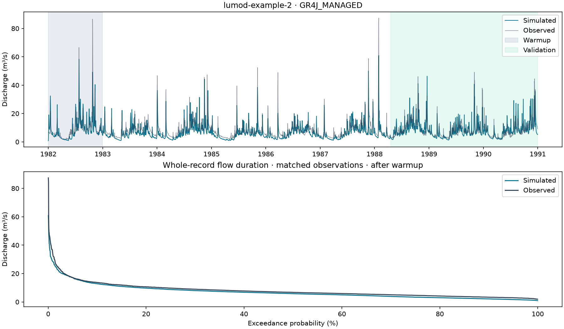
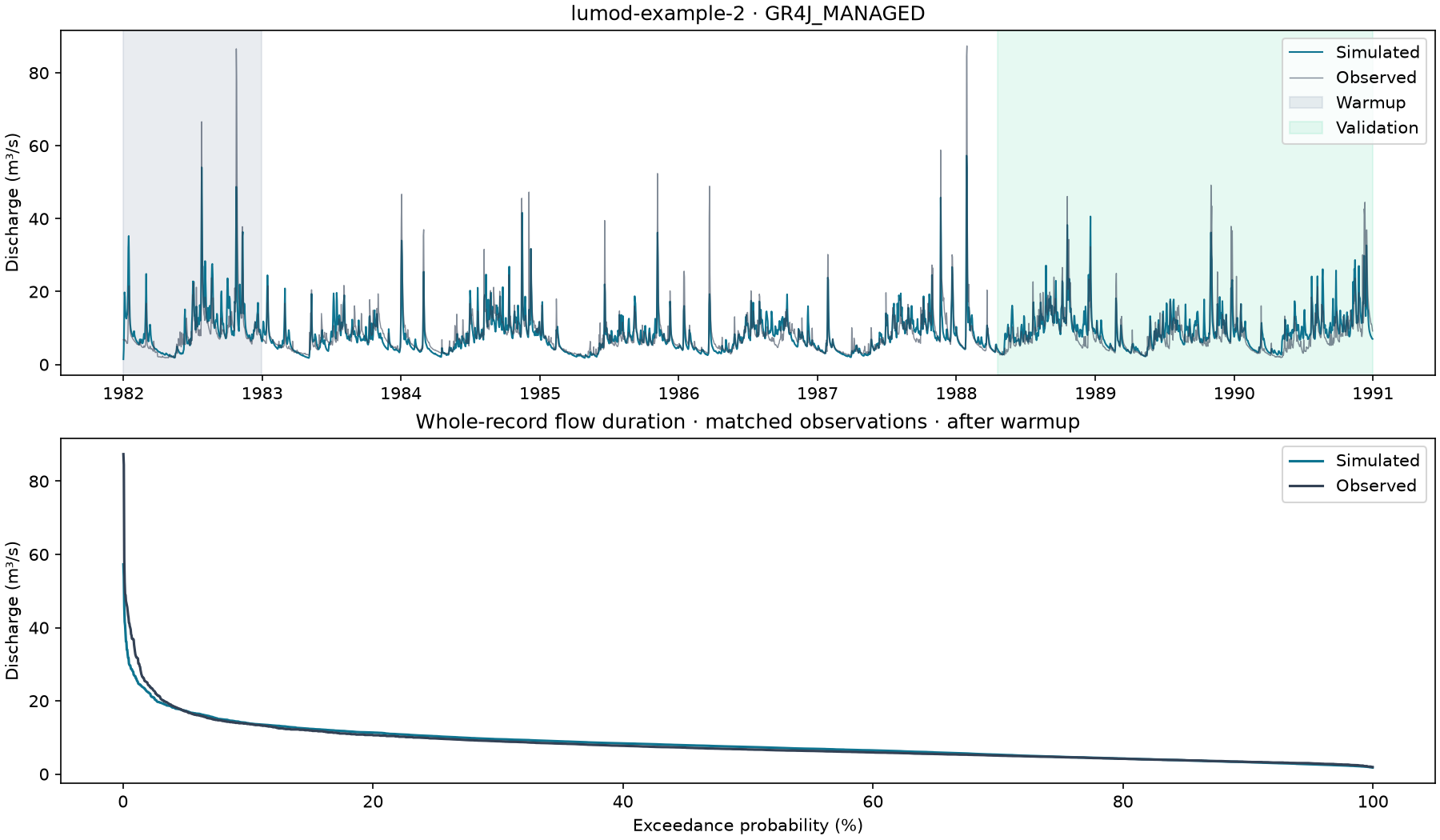
The executed scenario assumes 10,000 residents, irrigation on 5% of basin area with 60% of irrigation demand assigned to surface water and 40% to groundwater, and 500 m³/day industrial demand. Initial aquifer storage is 10 mm of catchment-equivalent water. The record contains 3,287 daily steps. Hydrological parameters were fitted; the withdrawal assumptions were fixed.

Search	Training NSE	Validation NSE	Validation KGE
DE	0.7050	0.6172	0.7421
LHS	0.6296	0.5590	0.7448
Multi-start DE	0.7149	0.6034	0.7184

These are limited-budget demonstrations: DE uses 10 iterations and population multiplier 5; LHS uses 100 samples; multi-start uses seeds 42 and 43. Warmup is 365 days and the chronological training fraction is 70%. Results do not establish that this managed representation improves on an unmanaged model.

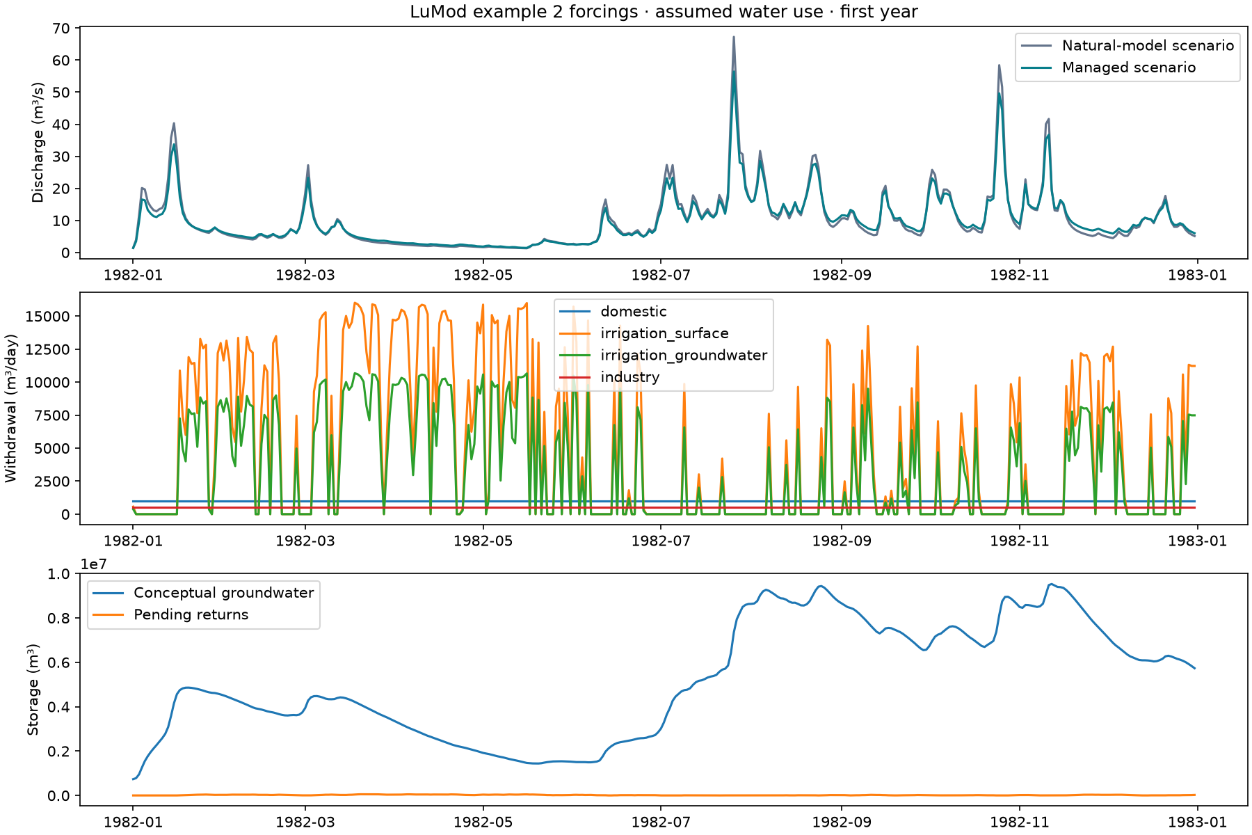
Natural-model and managed scenarios, sector withdrawals and stores

View fitted hydrographs: DE, LHS, multi-start. Download scenario assumptions and results and water-parameter Morris/Sobol results.

The maximum daily managed-water balance error was \(1.86\times10^{-9}\) m³. One local warmed run of priority accounting processed 3,287 days in about 0.8 ms; LP processed the first 365 days in about 0.66 s. These timings include the accounting API and table creation, but exclude hydrological simulation, calibration and initial compilation. They are not cross-machine benchmarks or a same-duration comparison. The network’s total balance residual was about \(-1.42\times10^{-7}\) m³, including end-of-record transit storage.

Scientific scope and sources

The aquifer is a lumped linear store, not native HBV groundwater storage or a spatial aquifer solution. Partitioning already-routed model runoff into a new store changes timing; partition/recession require independent justification. Well distance, aquifer transmissivity, drawdown, streambed resistance and spatial pumping impacts require a groundwater model such as MODFLOW or appropriate analytical depletion solutions.

The implementation is original BasinForge code. Scientific design references:

CWatM water demand: sector demands, consumption and returns.
PCR-GLOBWB 2: integrated withdrawals and water availability.
WaterGAP 2.2d: separate surface/groundwater abstractions and returns.
Pywr: network allocation using linear programming.
USGS streamflow depletion: limits of simplified pumping representations.

Tests cover hand-calculated cases, both allocators, randomized daily mass balances, depletion/returns, reservoir evaporation/releases, network transit, parallel/shared fitting and scenario-sensitive fingerprints. These establish numerical contracts, not predictive validity for a particular basin.